The example in this tutorial is taken from the classical textbook by N. van Kampen (1981): Stochastic processes in physics and chemistry, pp. 273-277, North-Holland. The results can be derived analytically and thus can be used to verify MuMoT’s output.
This is an educational example of to derive and work with a multivariate Master equation. It describes a chemical reaction in an open system and involves two reactants, $X$ and $Y$.
Let’s get started!
Model definition and basic model exploration
model1 = mumot.parseModel(r"""
(A) -> X : \alpha
X + X -> Y + \emptyset : \gamma
Y -> (B) : \beta
""")
The above input cell defines our model. If you went through the Getting started tutorial before you will have noticed the different way to define a model. Here, the advantage is that we do not need an absolute cell reference as in the other example. Note we did two steps in one - defining and parsing our model1.
To see the reactions in a nicer format, let’s look at them with the show() command:
model1.show()
$\displaystyle (A) \xrightarrow{\alpha}X $
$\displaystyle X + X \xrightarrow{\gamma}Y + \emptyset $
$\displaystyle Y \xrightarrow{\beta}(B) $
Here we have told MuMoT that $A$ and $B$ are constant reactants by putting them in parentheses, and the $\emptyset$-symbol indicates that we have an open system.
We can now derive the ODEs governing the deterministic dynamics of the system using …
model1.showODEs(method='vanKampen')
$\displaystyle \frac{d}{d t} \Phi_X := \Phi_A \alpha - 2 \Phi_X^2 \gamma$
$\displaystyle \frac{d}{d t} \Phi_Y := \Phi_X^2 \gamma - \Phi_Y \beta$
This is a bit different than what you have seen in the Getting started tutorial tutorial. Here we used the keyword method='vanKampen'. The effect of this is that the ODEs are derived via a van Kampen expansion (or system size expansion). We will get back to this later. To compare with the default method we can simply omit the keyword and use …
model1.showODEs()
$\displaystyle \displaystyle \frac{\textrm{d}Y}{\textrm{d}t} := X^{2} \gamma - Y \beta$
$\displaystyle \displaystyle \frac{\textrm{d}X}{\textrm{d}t} := A \alpha - 2 X^{2} \gamma$
You can see that the only difference is the symbol $\Phi$, which denotes concentrations throughout MuMoT. Concentrations or proportions are the quantities naturally arising from the van Kampen expansion.
To get an idea of what the dynamics in the system look like, we can numerically integrate the ODEs …
evol1 = model1.integrate(initWidgets={'initialState': {'X': [0.5,0,1,0.1], 'Y': [0.5,0,1,0.1]},
'maxTime': [5,3,20,1]},
legend_loc='center right')
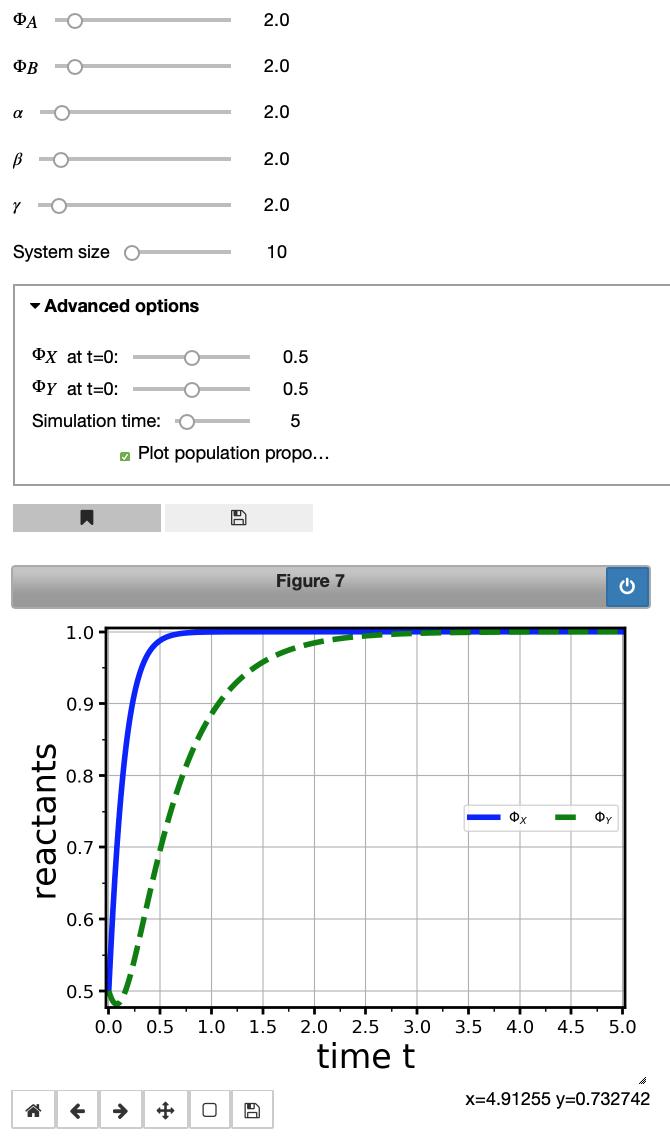
At this point, you might want to play with sliders and see how the plot changes. Also, you could investigate the expression in the input cell and check the effect in the Advanced options tab. Right, we changed the values on the slider. For more information on the options available, we refer to the comprehensive User Manual available on the MuMoT project page on GitHub or alternatively via this link on MyBinder (no installation necessary). Also note that we ticked the Plot population proportions box in the Advanced options tab.
Next, we might be interested to get some information on the fluctuations in the system. Remember the numerical integration in the plot above relates to the macroscopic equations that do not contain any noise. It describes how the system evolves on avarage. However, depending on the system size fluctuations may be non-negligible (the smaller the system size the larger the fluctuations).
Van Kampen expansion
Our first step to study noise inthe system is to derive the chemical Master equation, i.e. we ask MuMoT to do this calculation for us using …
model1.showMasterEquation()
$\displaystyle \frac{\partial}{\partial t} P{\left (X,Y,t \right )}:= \frac{A \alpha}{\overline{V}} ( \operatorname{E_{op}}{\left (X,-1 \right )} - 1 ) \overline{V} P{\left (X,Y,t \right )} + \gamma ( \operatorname{E_{op}}{\left (X,2 \right )} \operatorname{E_{op}}{\left (Y,-1 \right )} - 1 ) \frac{X \left(X - 1\right)}{\overline{V}} P{\left (X,Y,t \right )} + \beta ( \operatorname{E_{op}}{\left (Y,1 \right )} - 1 ) Y P{\left (X,Y,t \right )}$
In MuMoT we express the Master equation using step operators $E_{op}$, just as in van Kampen’s textbook. To derive expressions for the noise in the system, we make use of the linear noise approximation to derive a multivariate Fokker-Planck equation which is linear in the noise terms. This often cumbersome calculation can be automatically performed in MuMoT as follows:
model1.showFokkerPlanckEquation()
$\displaystyle \frac{\partial}{\partial t} P{\left (\eta_X,\eta_Y,t \right )} := \frac{\Phi_A \alpha \frac{\partial^{2}}{\partial \eta_X^{2}} P{\left (\eta_X,\eta_Y,t \right )}}{2} + 2 \Phi_X^{2} \gamma \frac{\partial^{2}}{\partial \eta_X^{2}} P{\left (\eta_X,\eta_Y,t \right )} + \frac{\Phi_X^{2} \gamma \frac{\partial^{2}}{\partial \eta_Y^{2}} P{\left (\eta_X,\eta_Y,t \right )}}{2} - 2 \Phi_X^{2} \gamma \frac{\partial^{2}}{\partial \eta_Y\partial \eta_X} P{\left (\eta_X,\eta_Y,t \right )} + 4 \Phi_X \eta_X \gamma \frac{\partial}{\partial \eta_X} P{\left (\eta_X,\eta_Y,t \right )} - 2 \Phi_X \eta_X \gamma \frac{\partial}{\partial \eta_Y} P{\left (\eta_X,\eta_Y,t \right )} + 4 \Phi_X \gamma P{\left (\eta_X,\eta_Y,t \right )} + \frac{\Phi_Y \beta \frac{\partial^{2}}{\partial \eta_Y^{2}} P{\left (\eta_X,\eta_Y,t \right )}}{2} + \beta \eta_Y \frac{\partial}{\partial \eta_Y} P{\left (\eta_X,\eta_Y,t \right )} + \beta P{\left (\eta_X,\eta_Y,t \right )}$
This expression is indeed identical to the analytical expression in van Kampens book (1981, p.275, Eq.(5.7)). In MuMoT we use the reserved symbol $\eta$ to represent noise and the index indicates the subsystem of reactants associated with it.
Brilliant! With just pressing a button the equation was derived in no time.
Although solving partial differential equations is not yet supported in MuMoT, we can do more useful stuff with the linear Fokker-Planck equation. For example, we can automatically derive the equations for the first- and second order moments …
model1.showNoiseEquations()
$\displaystyle \displaystyle \frac{\textrm{d}\left< \vphantom{Dg}\right.\eta_{X}\left. \vphantom{Dg}\right>}{\textrm{d}t} := - 4 \Phi_{X} \left< \vphantom{Dg}\right.\eta_{X}\left. \vphantom{Dg}\right> \gamma$
$\displaystyle \displaystyle \frac{\textrm{d}\left< \vphantom{Dg}\right.\eta_{Y}\left. \vphantom{Dg}\right>}{\textrm{d}t} := 2 \Phi_{X} \left< \vphantom{Dg}\right.\eta_{X}\left. \vphantom{Dg}\right> \gamma - \left< \vphantom{Dg}\right.\eta_{Y}\left. \vphantom{Dg}\right> \beta$
$\displaystyle \displaystyle \frac{\textrm{d}\left< \vphantom{Dg}\right.\eta_{X}^{2}\left. \vphantom{Dg}\right>}{\textrm{d}t} := \Phi_{A} \alpha + 4 \Phi_{X}^{2} \gamma - 8 \Phi_{X} \left< \vphantom{Dg}\right.\eta_{X}^{2}\left. \vphantom{Dg}\right> \gamma$
$\displaystyle \displaystyle \frac{\textrm{d}\left< \vphantom{Dg}\right.\eta_{X} \eta_{Y}\left. \vphantom{Dg}\right>}{\textrm{d}t} := - 2 \Phi_{X}^{2} \gamma + 2 \Phi_{X} \left< \vphantom{Dg}\right.\eta_{X}^{2}\left. \vphantom{Dg}\right> \gamma - \left< \vphantom{Dg}\right.\eta_{X} \eta_{Y}\left. \vphantom{Dg}\right> \left(4 \Phi_{X} \gamma + \beta\right)$
$\displaystyle \displaystyle \frac{\textrm{d}\left< \vphantom{Dg}\right.\eta_{Y}^{2}\left. \vphantom{Dg}\right>}{\textrm{d}t} := \Phi_{X}^{2} \gamma + 4 \Phi_{X} \left< \vphantom{Dg}\right.\eta_{X} \eta_{Y}\left. \vphantom{Dg}\right> \gamma + \Phi_{Y} \beta - 2 \left< \vphantom{Dg}\right.\eta_{Y}^{2}\left. \vphantom{Dg}\right> \beta$
and try to compute their solutions in the stationary state …
model1.showNoiseSolutions()
Stationary solutions of first and second order moments of noise:
$\displaystyle \left< \vphantom{Dg}\right.\eta_{Y}\left. \vphantom{Dg}\right>(t \to \infty):= 0$
$\displaystyle \left< \vphantom{Dg}\right.\eta_{X}\left. \vphantom{Dg}\right>(t \to \infty):= 0$
$\displaystyle \left< \vphantom{Dg}\right.\eta_{X}^{2}\left. \vphantom{Dg}\right>(t \to \infty) := \frac{\Phi_{A} \alpha}{8 \Phi_{X} \gamma} + \frac{\Phi_{X}}{2}$
$\displaystyle \left< \vphantom{Dg}\right.\eta_{Y}^{2}\left. \vphantom{Dg}\right>(t \to \infty) := \frac{\Phi_{A} \Phi_{X} \alpha \gamma + \Phi_{X}^{2} \beta \gamma + 4 \Phi_{X} \Phi_{Y} \beta \gamma + \Phi_{Y} \beta^{2}}{2 \beta \left(4 \Phi_{X} \gamma + \beta\right)}$
$\displaystyle \left< \vphantom{Dg}\right.\eta_{X} \eta_{Y}\left. \vphantom{Dg}\right>(t \to \infty) := \frac{\frac{\Phi_{A} \alpha}{4} - \Phi_{X}^{2} \gamma}{4 \Phi_{X} \gamma + \beta}$
If the equations are not too complicated, MuMoT can successfully derive analytical expressions, as in this example. We can also visualise the temporal evolution of noise-noise correlations using the following command:
Ncorr1 = model1.noiseCorrelations(maxTime=3, legend_loc='upper right', legend_fontsize=12)
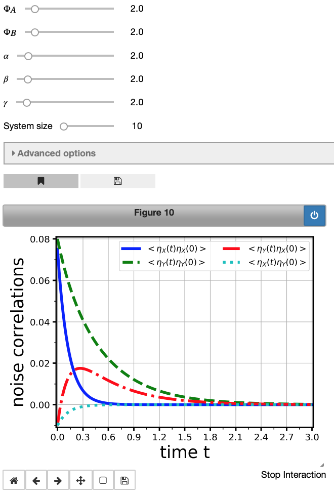
Fantastic! This produces a publication-ready figure with automatic labelling and legend generation (check the keywords in the input cell, too). Auto-correlations ($\eta_X(t) \eta_X(0)$ and $\eta_Y(t) \eta_Y(0)$) as well as cross-correlations ($\eta_X(t) \eta_Y(0)$ and $\eta_Y(t) \eta_X(0)$) are plotted.
More information can be found in the MuMoT User Manual (a Jupyter notebook). The quickest way to access this is by starting a server on MyBinder. Actually all you need to do is to follow this link and you can work with it straight away!