Getting started

MuMoT models are defined using the %%model keyword within a cell. The syntax is meant to be intuitive and all processes are described as chemical reaction-like expressions, including the reactants and reaction rates. Here is an example:

A + A -> A + U: s

where two particles of type $A$ interact, and one changes to type $U$, at rate $s$.

Now that we have a working model we can do some basic exploration. So, let MuMoT generate the set of Ordinary Differential Equations (ODEs) of our model1 for us.

model1.showODEs()

$\displaystyle \displaystyle \frac{\textrm{d}A}{\textrm{d}t} := - A B s + A U r_A - A a_A + U g_A$

$\displaystyle \displaystyle \frac{\textrm{d}U}{\textrm{d}t} := 2 A B s - A U r_A + A a_A - B U r_B + B a_B - U g_A - U g_B$

$\displaystyle \displaystyle \frac{\textrm{d}B}{\textrm{d}t} := - A B s + B U r_B - B a_B + U g_B$

We can analyse these equations further but before we do that let’s simplify them. One equation is redundant here because there is a constant number of individuals in the swarm during a decision, i.e. the system is conserved.

A simpler set of equations can be obtained using substitute() according to

model2 = model1.substitute('U = N - A - B')

To see that this indeed simplifies the ODEs we do (note that we created the new instance model2) …

model2.showODEs()

$\displaystyle \displaystyle \frac{\textrm{d}A}{\textrm{d}t} := - A B s - A a_A + A r_A \left(- B + \left(- A + N\right)\right) + g_A \left(- B + \left(- A + N\right)\right)$

$\displaystyle \displaystyle \frac{\textrm{d}B}{\textrm{d}t} := - A B s - B a_B + B r_B \left(- B + \left(- A + N\right)\right) + g_B \left(- B + \left(- A + N\right)\right)$

… and see that the number of equations was reduced from three to two. This is because the population of uncommitted bees has been replaced by $U=N-A-B$, where $N$ is the total number of bees which is a constant.

Now we can turn to more exciting graphical output and numerically integrate the ODEs using the MuMoT-method integrate()

int1 = model2.integrate()

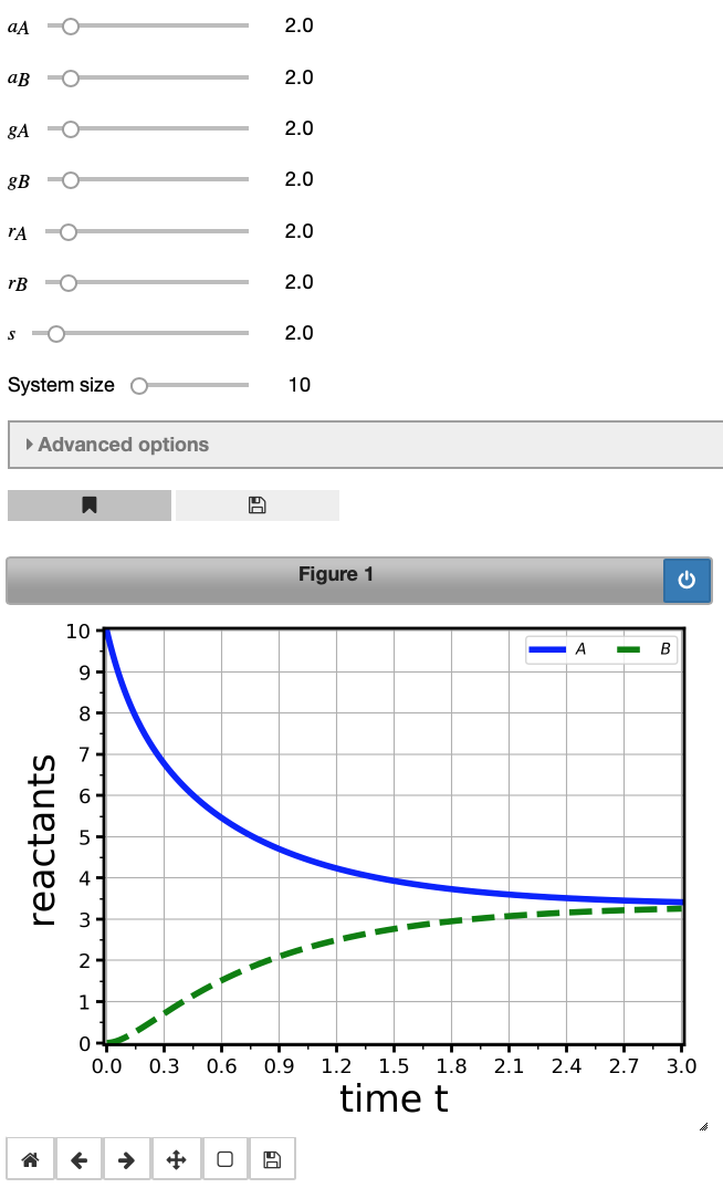
This should have created an interactive plot of the temporal evolution of populations over time. There are some sliders above the figure to manipulate this graph; MuMoT gives you a slider for every rate in the model, and by changing their values, you can see what happens to the behaviour of the system. There are more sliders in the Advanced options tab which you can try out.

Important information related to this plot can be retrieved be showing the logs with the showLogs command like so:

int1.showLogs(tail = True)

Showing last 3 of 3 log entries:
Starting numerical integration of ODE system with parameters (a_{A}=2.0), (a_{B}=2.0), (g_{A}=2.0), (g_{B}=2.0), (r_{A}=2.0), (r_{B}=2.0), (s=2.0), (initA=1.0), (initB=0.0), (initU=0.0), (maxTime=3.0), (conserved=True), (substitutedReactant=U), at 2019-04-05 17:49:23.730840
Last point on curve:

$\displaystyle A(t =3.0) = 3.4121$

$\displaystyle B(t =3.0) = 3.255$

As last part of this short introductory tutorial we will produce a vector of our system. This can be done using:

vector1 = model2.vector('A', 'B', showNoise = True)

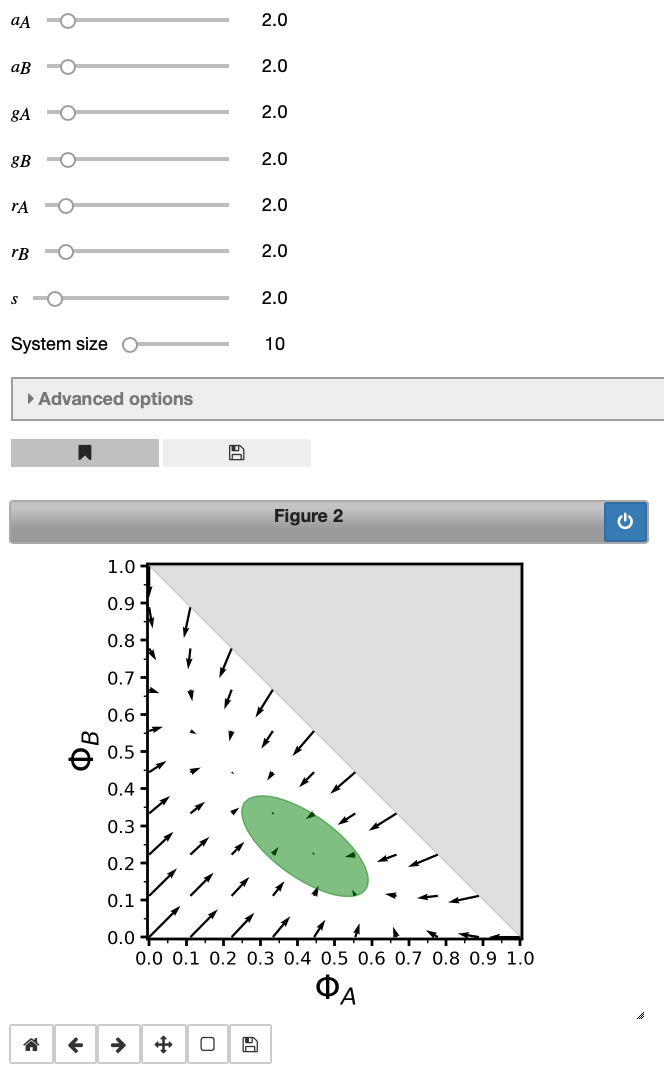
This vector plot depicts how the system evolves depending on the initial conditions. Proportions of bees in states $A$ and $B$ are labelled $\Phi_A$ and $\Phi_B$ - we use the upper-case Greek letter $\Phi$ to denote concentrations (proportions) and the reactants are added as indices. This is done throughout MuMoT and you will encounter this notation again when you work through more examples. Hence, upper-case $\Phi$ cannot be used as a user-defined symbol in MuMoT to avoid confusion. The green ellipse displays noise in the system due to a finite system size (change the system size slider above the plot and see how the ellipse changes; don’t increase the system size too much though, as this may increase computation time).

Again, model parameters may be altered via the sliders above the figure and useful information about the computation can be obtained using the showLogs() command:

vector1.showLogs(tail = True)

Showing last 3 of 3 log entries:
Starting 2d vector plot with parameters (a_{A}=2.0), (a_{B}=2.0), (g_{A}=2.0), (g_{B}=2.0), (r_{A}=2.0), (r_{B}=2.0), (s=2.0), (aggregateResults=True), (maxTime=2.0), (randomSeed=1680863739), (runs=20), at 2019-04-05 17:49:30.713976
Fixed point1:  A = -1.0000, B = -1.0000,  with eigenvalues:  4.0000, 8.0000,  and eigenvectors:  [-1.0000, 1.0000] and [1.0000, 1.0000]
Fixed point2:  A = 0.3333, B = 0.3333,  with eigenvalues:  -8.0000, -1.3333,  and eigenvectors:  [1.0000, 1.0000] and [-1.0000, 1.0000]